Design of a Machine Learning System to Predict the Thickness of a Melanoma Lesion in a Non-Invasive Way from Dermoscopic Images
Article information

Abstract
Objectives
Melanoma is the deadliest form of skin cancer, but it can be fully cured through early detection and treatment in 99% of cases. Our aim was to develop a non-invasive machine learning system that can predict the thickness of a melanoma lesion, which is a proxy for tumor progression, through dermoscopic images. This method can serve as a valuable tool in identifying urgent cases for treatment.
Methods
A modern convolutional neural network architecture (EfficientNet) was used to construct a model capable of classifying dermoscopic images of melanoma lesions into three distinct categories based on thickness. We incorporated techniques to reduce the impact of an imbalanced training dataset, enhanced the generalization capacity of the model through image augmentation, and utilized five-fold cross-validation to produce more reliable metrics.
Results
Our method achieved 71% balanced accuracy for three-way classification when trained on a small public dataset of 247 melanoma images. We also presented performance projections for larger training datasets.
Conclusions
Our model represents a new state-of-the-art method for classifying melanoma thicknesses. Performance can be further optimized by expanding training datasets and utilizing model ensembles. We have shown that earlier claims of higher performance were mistaken due to data leakage during the evaluation process.
I. Introduction
According to the American Cancer Society, skin cancer is the fifth most common type of cancer in the United States, of which malignant melanoma is the deadliest. Early detection plays a crucial role in cancer, as cancer progression can significantly affect mortality rates. Melanoma has a 5-year relative survival rate of 99% when confined to the skin, but the survival rate drops to 27% when it advances and metastasizes to vital organs [1].
With advances in machine learning and image processing algorithms over the past decade, including techniques like convolutional neural networks, image recognition tasks have achieved almost human-like and sometimes even superhuman results [2]. Unsurprisingly, many studies have aimed to develop software that can recognize malignant melanoma in a non-invasive manner using dermoscopic images of skin lesions, thanks to these algorithms. Machine learning algorithms require training data, for which a considerable amount of public data is available, especially associated with the International Skin Imaging Collaboration (ISIC) (see, e.g., [3–6]). This availability has accelerated model development, making it possible to apply these techniques to early melanoma detection, potentially saving human lives by reducing the need for trained professional dermatologists, who may be costly or unavailable in remote areas around the world.
Diagnosing skin cancer is the first and arguably the most important step toward curing the disease, but determining the severity and progression of the tumor can be just as crucial for treatment planning. Artificial intelligence can provide a solution to this problem. The thickness of melanoma lesions is the most important predictor of their prognosis [7]. However, current clinical procedures to evaluate lesion depth involve biopsy for pathological examination. Therefore, developing a system that can estimate melanoma thickness non-invasively from dermoscopic images can prioritize the most critical cases.
This task presents a unique challenge as there is an abundance of visual data regarding the type of skin lesion, but a scarcity of information about its depth. Consequently, only a few attempts have been made to create a machine learning model for this task due to the severely limited availability of data required for training purposes.
Rubegni et al. [8] conducted a study in 2010 wherein they employed logistic regression for estimating the thickness of melanomas. The data were divided into two categories: those with depths greater than 1 mm and those with depths less than 1 mm. Forty-nine independent features, such as the area and color gradient of skin lesion images, were chosen to train the model. The researchers carried out the experiments on a private dataset consisting of 141 melanoma images, out of which 108 had a thickness of less than 1 mm while 33 had a greater thickness. The study achieved an accuracy rate of 86.5%, with a specificity of 89.8% and sensitivity of 75.7%.
Saez et al. [9] used binary and multiclass approaches to classify melanoma thickness. They employed several feature extraction techniques, such as shape, color, and texture, which yielded 81 distinct values per image. Various machine learning models were trained using these values. Among them, logistic regression with initial variables and product units achieved 77.6% accuracy for the binary classification and 68.4% for three-class classification. However, these models showed a tendency to favor classes that were over-represented in the dataset, owing to class imbalance, which adversely affected the model’s mean specificity.
In a follow-up paper [10], the same techniques were applied to five classes. In addition to the three melanoma thickness classes, the study also incorporated non-melanoma and melanoma in situ images. An accuracy of 68.5% on these classes was achieved, although a bias toward the over-represented class persisted.
In 2019, Jaworek-Korjakowska et al. [11] presented a method that utilized convolutional neural networks with VGG-19 architecture as the backbone and employed transfer learning. They also used the synthetic minority oversampling technique (SMOTE) to address class imbalance in the dataset by generating synthetic images for the under-represented classes [12]. The authors trained the model on a dataset with 244 images separated into three thickness classes and achieved an accuracy of 87.2% and an F1-score of 83.4%. However, upon further examination of the presented training and testing pipeline, we identified an error that might cause leakage, resulting in an overly optimistic score for the model. We elaborate on this point in more detail in Section IV (Discussion).
This paper presents a method for categorizing melanoma skin lesions into three different thickness categories. These categories include thin lesions with a depth of less than 0.76 mm or those that are melanoma in situ; intermediate melanomas with depths between 0.76 mm and 1.5 mm; and thick melanomas with depths exceeding 1.5 mm. Despite being trained on a small dataset, our model outperformed previous results. We also present a projection of the performance of this method for larger training datasets.
II. Methods
1. Dataset and Preprocessing
We use the dermoscopic image set of the publicly available Derm7pt dataset [13], which contains information on lesion depth. However, many of the images contain objects like oil blobs, hair, and measuring marks that are not part of the lesion. To minimize the impact of these artifacts [11], we implemented uniform preprocessing by cropping around the lesion and resizing the image to a 1:1 ratio. This approach helped eliminate most of the obstructing objects while ensuring that all the lesions had a comparable size in the preprocessed images. We conducted experiments with and without cropping and found that cropping achieved superior results.
2. Model Architecture
Because the dataset is relatively small, we employed transfer learning, as has been done in previous research [11]. We began training with a model that was pretrained on the ImageNet dataset. However, we replaced the VGG-19 architecture with the more up-to-date and reliable EfficientNet-B4 architecture [14] as the backbone. These EfficientNet-based models are able to achieve exceptional accuracy on the ImageNet dataset while also being smaller and, as a result, faster than many other architectures.
3. Reducing the Effect of Class Imbalance
As shown in Table 1, the classes in the dataset had varying sizes. It is crucial to note that the least advanced class (“thin”) was the majority class in our case. If the class imbalance is not addressed, the model may exhibit a bias toward the majority class, leading to a higher incidence of misclassification, particularly of advanced melanomas being misclassified as “thin” rather than the reverse. Such errors can have serious complications in applications where urgent cases require prioritization, causing delays in treatment.

Jaworek-Korjakowska et al. [11] employed SMOTE to address this issue. However, as we will show in Section IV (Discussion), this technique could lead to data leakage. Instead, we opted to use a combination of methods.
Weighted class training is one of the most widely used and straightforward techniques to combat class imbalance. The technique involves assigning a weight to each class that is inversely proportional to its frequency in the dataset. During training, the learning rate is adjusted for each sample based on its class weight.
Initially, the dataset consisted of four distinct classes, but we narrowed down our classification problem to three categories for melanoma progression. This was achieved by combining the classes of melanoma in situ and melanoma depth less than 0.76 mm since in situ melanomas, where the tumor has not spread beyond its original location in the epidermis, generally have a depth of less than 0.76 mm. There is no clear distinction between the classes, as both are early stages. However, we can make use of the finer category resolution by training our model on the original four classes and then merging them during the validation phase. This way, the training classes have a more balanced distribution. Even though the overall accuracy is higher while training on three classes, the balanced accuracy, which eliminates bias towards the majority class, is higher while training on four classes.
4. Data Augmentation
To ensure better generalization of the model, extensive data augmentation was applied to the images during training, given the limited size of the dataset. The following steps were followed in combination.
• Transposition: the rows and columns of the image were swapped with a probability of 0.5;
• Vertical and horizontal flip: each was applied independently with a probability of 0.5;
• Random brightness and contrast change: both were carried out independently with a 20% limit in the positive and negative direction and applied with a probability of 0.75;
• Blur: applied with a probability of 0.7 using either motion blur, median blur, Gaussian blur, or Gaussian noise;
• Distortion: applied with a probability of 0.7 using optical distortion, grid distortion, or elastic distortion;
• Random HSV (hue, saturation, and value) shift: each with a probability of 0.5; with a hue shift limit of 10, a saturation shift limit of 20, and a value shift limit of 10 in both the positive and negative direction;
• Random shifting: applied with a probability of 0.85 and a shift limit of 0.1 (in units of image length);
• Random scaling: with a probability of 0.85, rescaled with a random scale factor between 0.9 and 1.1; and
• Random rotation: with a probability of 0.85, the image was rotated by a random angle (±15°).
5. Training and Validation
During training and validation, the images were resized to a uniform 380×380 pixel size. We trained the model for 15 epochs using a batch size of 25, the Adam optimizer, and the cosine annealed learning rate scheduler with an initial learning rate of 3×10⁻⁵. Five-fold cross-validation was also used to validate the model to obtain more reliable metrics of its performance [15]. The values in Section III (Results) reflect the average performance of the model across the folds on the validation set of each fold.
6. Metrics
When performing classification, accuracy is the most natural metric to use. This measures the proportion of validation samples that are predicted correctly. Nonetheless, when dealing with datasets that are imbalanced, such a metric may be less informative because a model that predicts the majority class all the time can obtain a high score. Additionally, it is relevant to differentiate between type I error and type II error (false positives and false negatives, respectively). Therefore, in addition to accuracy, we considered balanced accuracy, which is defined as the accuracy measured per class, averaged over the classes as
where I is the indicator function and c(x) and ĉ (x) are the true and predicted classes, respectively, for the validation sample x; this quantity can also be considered as the average true positive rate (ATPR) (for a given class, “positive” is that class, and an average is then taken over the classes). The average true negative rate (ATNR) is defined similarly:
where for a given class k, the “negative” is any class except k; due to this definition, this multiclass metric tends to be high. Finally, the F1-score generalized to the multiclass context is the harmonic mean of the multiclass sensitivity (ATPR) and multiclass precision (defined similarly to the quantities above).
III. Results
1. Performance Measurements
Table 2 presents the accuracy and balanced accuracy of our method for a three-class classification problem compared to the previous approach. Our comparison includes the approach of Jaworek-Korjakowska et al. [11], which excluded data leakage, along with the two top-performing models of Saez et al. [9]. We calculated the metrics for these models using the provided confusion matrices from the paper. Table 3 presents a comparison using various classifier backbones. The results are commented upon in Section IV-1.

Our results compared with previous methods in the literature
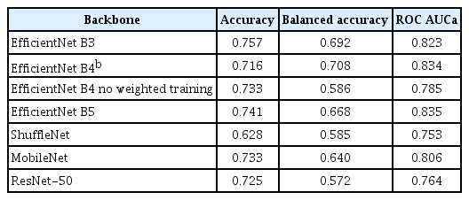
Comparison of our model using different backbones, when training on four classes and validating on three classes
2. Performance Projection for a Larger Dataset
While the method presented for this problem outperforms prior methods in terms of performance, it is still inadequate for real-world applications. Due to the limited amount of data required to train a machine learning model, this task is extremely challenging. By collecting additional data, the performance of the method can be significantly improved as the model has more examples to generalize. To determine the amount of additional data required for improved performance, we assessed the model’s performance on smaller subsets of the data and extrapolated our findings.
Random sampling was performed on the images of the smaller datasets extracted from the original dataset, while ensuring that the ratio of the different classes remained constant as it was initially. In total, 16 distinct subsets were formed, with varying sizes. The smallest subset size was 25% of the original dataset, while the other subsets’ sizes gradually increased in increments of 5% up to 95%. We trained a model using our method on each dataset and performed five-fold cross-validation for the balanced accuracy metric.
To estimate performance for a more extensive dataset, we used an exponential function that would ideally reach a perfect score:
where x = N/N0 is the ratio of the size of the dataset N and the size of the original dataset (N0 = 247). The mean squared error was minimized by parameter values of a = −0.68 and b = −0.81.
Figure 1 shows the balanced accuracies of each subset as a function of size ratio and the reverse exponential curve fit. The chosen fitting function is reasonable, and from the plotted data, it is apparent that a more extensive dataset could lead to even higher benchmark scores.

Balanced accuracy of each subset as a function of the dataset size ratio and the reverse exponential curve fit.
IV. Discussion
1. Model Performance
As can be observed from Table 2, our method outperformed the previous state-of-the-art results in both traditional accuracy and balanced accuracy, except for the results reported by Jaworek-Korjakowska et al. [11]. We will scrutinize those results in detail in the next section. The highest balanced accuracy was attained when the method was trained on four classes and used to predict the partially merged three classes. The problem of categorizing into four categories is a more complex problem, which is evident from the numerical values.
Although it is commonly believed that stronger backbones perform better, this is not always the case, as can be seen in Table 3. Multiple factors might explain why the balanced accuracy obtained with EfficientNet-B5 was lower than that of B4: (1) the larger backbone (B5) contained more parameters, making it more liable to overtraining, especially for the small dataset we used; (2) the uncertainty in the performance values is large for a small dataset, even if cross-validation is used (for balanced accuracy, the error contribution of the minority classes can be especially large); and (3) our hyper-parameters were optimized more heavily for B4. We note that uncertainties can, in principle, be evaluated by conducting a series of independent training sessions with varying random dataset splits for cross-validation, and then comparing the outcomes [16].
2. Data Leakage in [11] and its Reproduction
This section presents our analysis demonstrating that the high scores reported by Jaworek-Korjakowska et al. [11] were most probably due to data leakage.
Jaworek-Korjakowska et al. [11] offered a thorough account of the pipeline they used for both training and validating purposes in their paper. Following image processing such as cropping and resizing, each image was allocated to one of three thickness classes. These categories were identical to ours, and our datasets shared similarities (Table 1).
The authors used the SMOTE oversampling technique [12] to deal with the class imbalance in the preprocessed data. They generated new samples for minority classes based on existing data in the given class, resulting in equal-size classes. Once the classes were balanced, the data were split into two parts: training data (to train the model) and testing data (for performance evaluation).
In machine learning, it is common practice to use separate data for training and for validation [15]. This eliminates the possibility of “memorizing” the dataset, allowing an accurate estimation of model performance on new, unseen data. However, the training and validation datasets must be entirely independent for this to work. Data leakage arises when information about the validation data is incorporated into the training procedure, providing an unrealistic and overly optimistic estimate of the model’s performance. This leakage usually occurs when pre-processing the training and testing data jointly [17].
The above problem is an issue for that paper, as the authors utilized SMOTE oversampling prior to dividing the data. SMOTE functions by generating synthetic data from a few representative samples from the same class to increase the minority classes to the size of the most prominent class. Although it is an appropriate method for low-dimensional data, SMOTE can create nearly identical copies of specific pre-existing images with visual data since the dimensionality of the problem space tends to be extremely high.
To illustrate, we applied the SMOTE algorithm to a collection of melanoma images. The minority class in the dataset comprised 28 samples, which we augmented by adding 74 artificially generated images, resulting in a total of 102 images. These numbers correspond to the size of the smallest minority class and the majority class in the dataset that we employed for our tests, respectively. Figure 2 depicts two images: one of them belonged to the original dataset, whereas the other was produced by the SMOTE algorithm. Notably, the newly created image bears significant similarity to the original one. It can clearly be seen that by splitting the dataset after the oversampling step, the training set could include samples that have been influenced by some validation samples, resulting in a misleadingly high score during evaluation.

Comparison between an original dermoscopic image (A) and a SMOTE-generated image (B). The two images are very similar, but not identical; for example, the curved line (piece of hair) on the right-hand side of the generated image is copied from a different sample. The original image is from the ISIC2018 Task-1 Challenge dataset (https://challenge.isic-archive.com/data/) provided with a CC0 license. SMOTE: synthetic minority oversampling technique.
To prove our hypothesis regarding data leakage, we implemented the algorithm while carefully following every step. We then modified the algorithm slightly by only applying the SMOTE oversampling to the training set, while making sure not to mix the training and validation samples. We used five-fold cross-validation to obtain a more stable evaluation of the model’s actual performance.
In this experiment, we utilized the Derm7pt dataset [13], which bears resemblances to the dataset presented by Jaworek-Korjakowska et al. [11] (Table 1). To enable three-class classification [11], melanoma in situ and melanoma depth of 0.76 mm were merged.
Table 4 shows the performance of the method presented in this paper and the result we obtained using this method with or without data leakage (i.e., where the oversampling step was performed before the dataset splitting). Jaworek-Korjakowska et al. [11] provided accuracy, the ATPR, the ATNR, and the F1-score as metrics to measure performance; thus, we compared these scores in our experiment.
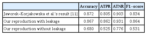
Our results with data leakage were similar to those reported in the original paper and, in some cases, even surpassed them. However, when we tested the method without data leakage by only validating on images the model did not see during training, we obtained much lower values. This was particularly evident in the ATPR and F1-score, which, unlike accuracy, give equal weight to each class and provide a more meaningful metric for imbalanced datasets.
3. Summary and Outlook
In conclusion, this paper discussed the possibility of estimating the progression of melanomas. We presented a method that can predict the thickness of skin cancer from dermoscopic images and categorize it into three classes accurately, with an accuracy of 0.716 and a balanced accuracy of 0.708, which is better than previous state-of-the-art methods. While this performance may not be adequate for real-world clinical use, we demonstrated that there is potential for improvement by using additional training data to generate synthetic data by utilizing models such as generative adversarial networks (GANs) [18] or by utilizing larger datasets more effectively. The training and validation dataset we used included approximately 250 samples, while excellent public datasets are available with tens of thousands of samples without any information about thickness. Additionally, collecting data with exact thickness values instead of predefined classes would enable us to consider thickness prediction as a regression task, resulting in more precise predictions.
Notes
Conflict of Interest
No potential conflict of interest relevant to this article was reported.
Acknowledgments
This study was supported by the Application Domain Specific Highly Reliable IT Solutions project implemented with the support provided from the National Research, Development and Innovation Fund of Hungary, financed under the Thematic Excellence Programme TKP2020-NKA-06 (National Challenges Subprogramme) funding scheme, and the European Union project RRF-2.3.1-21-2022-00004 within the framework of the Artificial Intelligence National Laboratory. The authors thank to Robert Bosch Ltd., Budapest, Hungary for their generous support to the Department of Artificial Intelligence.